

Reducing warranty costs of Valtra's tractors with Machine Learning
This time in Advian's blog we will take a deep dive into technical, when Matti Karppanen writes about the best tools and practices for machine learning.
Matti is a former professional poker player and a top-notch data scientist, whose specialties lie in linear algebra, neural networks and deep learning. Matti has been a key player in many challenging analytics projects. In addition to machine learning, Matti is highly skilled in understanding the real customer needs and problems.
Introduction
There is a multitude of tools, methods, libraries, and algorithms available free, in open source, for tasks related to machine learning. It is difficult to keep track of what is available. Furthermore, the field advances rapidly and it is also a challenge to keep up to date with all new developments.
This is our suggestion on what a machine learning practitioner could use in some of the subtasks of data analysis and machine learning modeling to improve their workflow. We limit the focus of this article on tabular data. NLP or computer vision will not be discussed.
Exploratory data analysis (EDA)
Our primary recommendation is to use the Sweetviz library in Python. Sweetviz allows you to make a thorough survey of a data frame in a few lines of code and a glance. This guide by the Sweetviz creator shows the potential.
Loading and saving data
CSVs and other text files can get cumbersome when the size of the data grows. In this case, we recommend Apache Parquet. It’s a compressed tabular data format that is both considerably faster to read and write, as well as more compact in terms of file size than plain CSVs are. The improvements for a 4Gb CSV file we had recently were a 25 times smaller parquet file that was 8 times faster to read with Pandas.
Missing value imputation
Don’t delete the rows. That’s throwing away information.
Imputing mean, mode, or median is common, and plain wrong. You’ll have to manually and inefficiently think and choose the correct between the three options for each column based on distribution and domain knowledge. And even if you choose the best one of these for your column, you often end up with a considerable portion (often over 10%) of your data having the same value. This does not help any machine learning model to learn very effectively and besides, makes your distribution artificially narrow. Finally and most importantly, using a central tendency parameter as your imputed value assumes the column is uncorrelated with all other columns. This is almost never true with real life data and you’ll end up with unlikely or even physically impossible values for some rows with extreme values in correlated columns.
Consider a dataset of apartments, which includes columns for area and number of rooms. The number of rooms column has some missing values. The mean number of rooms is 3.14, while median and mode are both 3. We would not want to impute any of these values in rows where apartment size is 15m2 or 300m2, would we?
The solution is to use a regression model specifically designed to impute missing values. Use IterativeImputer from scikit-learn, or MissForest on R. This benchmark on scikit-learn’s website has BayesianRidge as the top candidate for the underlaying model to be used with IterativeImputer. Remember to use indicator variables to mark the rows that had the missing value. This is information that the model can use if the missing values were not missing at random.
Data Scaling and Transformation
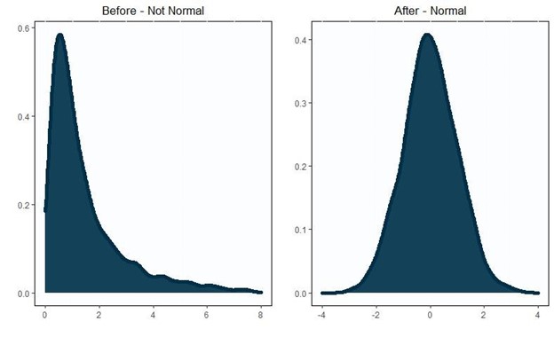
If the data does not follow a normal distribution, shifting and scaling to mean 0 and standard deviation 1 would not alter the shape and make the data normal. To actually transform non-normal data to normal, we have two options: Power Transforms and rank-based Inverse Normal Transformations (INT). Power Transforms are implemented directly in scikit-learn. To perform INT in scikit-learn, assign output_distibution="normal" in QuantileTransformer.
Hyperparameter optimization
Tree-structured Parzen Estimators (TPE) is the state-of-the-art for Bayesian optimization algorithms.
Covariance Matrix Adaptation Evolution Strategy (CMA-ES) is the state-of-the-art for evolutionary optimization algorithms.
Comparing the two, TPE tends to find a good set of hyperparameters with a smaller number of iterations, but CMA-ES tends to be better in actually finding the global optimum.
We recommend the hyperparameter optimization Python library Optuna, which implements both these algorithms.
Optuna can be used to code external hyperparameters and scoring metrics. Consider using training time, memory used, and model size on disk as weighted penalties to the evaluation metric when optimizing hyperparameters. Examples of external hyperparamers: number of features, multicollinearity threshold, imputation method, scaling method.
Metrics and loss functions
Metrics are used to compare trained model performance on the test set. Loss functions are used to calculate gradients while training a model. These need not to be the same often should not be.
Binary classification
The loss function is going to be logloss. It’s fine and often cannot even be changed.
For classification metrics, we recommend MCC in addition to ROC AUC and PR AUC. We assume the reader is familiar with both of the AUCs. If not, please click the link.
The Matthews Correlation Coefficient (MCC) measures the correlation of true classes with the predicted labels. MCC generates a high score only if the classifier correctly predicted most of the positive data instances and most of the negative data instances, and if most of its positive predictions and most of its negative predictions are correct. It also is symmetrical, meaning the choice of the positive label does not alter the score.
These papers by Chicco et al. contain clear and readable comparisons of MCC to other widely used classification metrics.
MCC also has an extension for multiclass classification.
Regression
Mean Squared Error is very sensitive to outliers. We have found that’s not ideal for model training very often.
Mean Absolute Error is not differentiable at the origin. The most widely used machine learning algorithms use gradients to find a minimum, so this is a problem.
Huber loss is a convex curve for small values near the origin and linear for large values. It’s included in both pytorch and tensorflow, and is our recommendation for those frameworks.
However, algorithms based on Gradient Boosted Trees use Hessians, meaning that you need second order partial derivatives. Huber loss is not second order differentiable. To circumvent this issue, XGBoost provides pseudohuber, while LightGBM and CatBoost provide a metric called “fair loss”. Both of these are second order differentiable functions which are insensitive to outliers.


